Of Particular Significance

Tag: fields

Today I continue with my series of posts on fields, strings and predictions.

During the 1980s, as I discussed in the previous post in this series, string theorists learned that of all the possible string theories that one could imagine, there were only five that were mathematically consistent.

What they learned in the first half of the 1990s, culminating in early 1995, is that all five string theories are actually little corners of a single, more encompassing, and still somewhat mysterious theory. In other words, after 30 years of studying various types of theories with strings in them, they ended up with just one!

On the one hand, that sort of sounds like a flop — all that work, by all those people, over two decades, and all we got for our efforts was one new theory?

On the other hand, it’s very tempting to think that the reason that everyone ended up converging on the same theory is that maybe it’s the only consistent theory of quantum gravity! At this point there’s no way to know for sure, but so far there’s no evidence against that possibility.  Certainly its a popular idea among string theorists.

This unique theory is called “M theory” today; we don’t know a better name, because we don’t really know what it is. We don’t know what it describes in general. We don’t know a principle by which to define it. Sometimes it is called “string/M theory” to remind us that it is string theory in certain corners.

Fig. 1: M theory is a set of equations that, depending on how they are used, can describe all known consistent  string theories and 11-dimensional supergravity, as well as many more complex and harder to understand things.  Only at the corners does it give the relatively simple string theories described in my previous post.
Fig. 1: A famous but very schematic image of M theory, which is a set of equations that, depending on how they are used, can describe universes whose particles and forces are given by any one of the known consistent string theories or by 11-dimensional supergravity.   Only at the corners does it give the relatively simple string theories described in my previous post.  More generally, away from the corners, it describes much more complicated and poorly understood types of worlds.

Note that M theory is very different in one key respect from quantum field theory.  As I described in the second post in this series, “quantum field theory” is the term that describes the general case; “a quantum field theory” is a specific example within the infinite number of “quantum field theories”. But there’s no analogue of this distinction for M theory. M theory is (as far as anyone can discern) a unique theory; it is both the general and the specific case.  There is no category of “M theories”. However, this uniqueness, while remarkable, is not quite as profound as it might sound… for a reason I’ll return to in a future post.

Incidentally, the relationship between the five apparently very different string theories that appear in M theory is similar to the surprising relationships among various field theories that I described in this post. It’s not at all obvious that each string theory is related to the other four… which is why it took some time, and a very roundabout route involving the study of black holes and their generalizations to black strings and black branes, for this relationship to become clear.

But as it did become clear, it was realized that “M theory” (or “string/M theory”, as it is sometimes called) is not merely, or even mainly, a theory of strings; it’s much richer than that. In one corner it is actually a theory with 10 spatial (11 space-time) dimensions; this is a theory with membranes rather than strings, one which we understand poorly. And in all of its corners, the theory has more than just strings; it has generalizations of membranes, called “branes” in general. [Yes, the joke’s been made already; the experts in this subject had indeed been brane-less for years.] Particles are zero-dimensional points; strings are one-dimensional wiggly lines; membranes are two-dimensional surfaces. In the ordinary three spatial dimensions we can observe, that’s all we’ve got. But in superstring theory, with nine spatial dimensions, one doesn’t stop there. There are three-dimensional branes, called three-branes for short; there are four-branes, five-branes, and on up to eight-branes. [There are even nine-branes too, which are really just a way of changing all of space. The story is rich and fascinating both physically and mathematically.] The pattern of the various types of branes — specifically, which ones are found in which corners of M theory, and the phenomena that occur when they intersect one another — is a fantastically elegant story that was worked out in the early-to-mid 1990s.

A brane on which a fundamental string can end is called a “D-brane”. Joe Polchinski is famous for having not only co-discovered these objects in the 1980s but for having recognized, in mid-1995, the wide-ranging role they play in the way the five different string theories are related to each other. I still remember vividly the profound effect that his 1995 paper had on the field. A postdoctoral researcher at the time, I was attending bi-weekly lectures by Ed Witten on the new developments of that year. I recall that at the lecture following Polchinski’s paper, Witten said something to the effect that everything he’d said in his presentations so far needed to be rethought. And over the next few months, it was.

DBranes
Fig. 2: In addition to fundamental strings (upper left), string theories can have D-branes, such as the D string (or D1-brane) shown at lower left, the D particle (or D0 brane) shown at lower right, or the D2-branes shown at right. There are also D3, D4, D5, D6, D7, D8 and D9 branes, along with NS5-branes, but since they have more than two spatial dimensions I can’t hope to draw them. There are no strings or D-branes, but there are M2-branes and M5- branes, in the 11-dimensional corner of M theory. A D-brane is an object where a fundamental string can end; therefore, in the presence of D-branes, a closed string can break into an open string with both ends on a D-brane (center and right).

The fact that string/M theory is more than just a theory of strings is strikingly similar to something known about quantum field theory for decades. Although quantum field theory was invented to understand particles in the context of Einstein’s special relativity, it turns out that it often describes more than particles. Field theory in three spatial dimensions can have string-like objects (often called “flux tubes”) and membrane-like objects (often called “domain walls”) and particle-like blobs (“magnetic monopoles”, “baryons”, and other structures). The simplest quantum field theories — those for which successive approximation works — are mainly theories of particles.  But flux tubes and domain walls and magnetic monopoles, which can’t be described in terms of particles, can show up even in those theories. So the complexities of M theory are perhaps not surprising. Yet it took physicists almost two decades to recognize that “branes” of various sorts are ubiquitous and essential in string/M theory. (We humans are pretty slow.)

Notably, there are contexts in which M theory exhibits no string-like objects at all. It’s the same with particles and fields; simple field theories have particles, but most field theories aren’t simple, and many complicated field theories don’t have particles. It can happen that the particles that would be observed in experiments may have nothing to do with the fields that appear in the equations of the theory; this was something I alluded to in this article. I also earlier described scale-invariant quantum field theories, which don’t have particles. Quantum field theories on curved space-time don’t have simple, straightforward notions of particles either. Quantum field theory is complex and rich and subtle, and we don’t fully understand it; I wrote seven posts about it in this series, and did little more than scratch the surface. String/M theory is even more complicated, so it will surely be quite a while before we understand it. But specifically, what this means is that what I told you in my last article about “simple superstring theories” is simply not always true. And that means that the first “vague prediction of string theory” that I described might not be reliable… no more than overall predictions of simple field theory, all of which are true in the context of simple field theories, but some of which are often false in more complex ones.

By the way, those of you who’ve read about string theory may wonder: where is supersymmetry in my discussion? Historically, in all these developments, the mathematics and physics of supersymmetry played an important role in making it easier to study and confirm the existence of these branes within string/M theory. However, the branes are present in the theory even when supersymmetry isn’t exact. One must not confuse the technically useful role of supersymmetry in clarifying how string/M theory works for a requirement that supersymmetry has to be an exact (or nearly-exact) symmetry for string/M theory to make sense at all. It’s just a lot harder to study string/M theory in the absence supersymmetry… something which is also true, though to a somewhat lesser extent, of quantum field theory.

To be continued… next, how are quantum field theory and M theory similar and different?

Picture of POSTED BY Matt Strassler

POSTED BY Matt Strassler

ON February 26, 2014

Appropriate for Advanced Non-Experts

[This is the seventh post in a series that begins here.]

In the last post in this series, I pointed out that there’s a lot about quantum field theory [the general case] that we don’t understand.  In particular there are many specific quantum field theories whose behavior we cannot calculate, and others whose existence we’re only partly sure of, since we can’t even write down equations for them. And I concluded with the remark that part of the reason we know about this last case is due to “supersymmetry”.

What’s the role of supersymmetry here? Most of the time you read about supersymmetry in the press, and on this website, it’s about the possible role of supersymmetry in addressing the naturalness problem of the Standard Model [which overlaps with and is almost identical to the hierarchy problem.] But actually (and I speak from personal experience here) one of the most powerful uses of supersymmetry has nothing to do with the naturalness problem at all.

The point is that quantum field theories that have supersymmetry are mathematically simpler than those that don’t. For certain physical questions — not all questions, by any means, but for some of the most interesting ones — it is sometimes possible to solve their equations exactly. And this makes it possible to learn far more about these quantum field theories than about their non-supersymmetric cousins.

Who cares? you might ask. Since supersymmetry isn’t part of the real world in our experiments, it seems of no use to study supersymmetric quantum field theories.

But that view would be deeply naive. It’s naive for three reasons. (more…)

Picture of POSTED BY Matt Strassler

POSTED BY Matt Strassler

ON November 20, 2013

For More Advanced Non-Experts

[This is part 6 of a series, which begins here.]

I’ve explained in earlier posts how we can calculate many things in the quantum field theory that is known as the “Standard Model” of particle physics, itself an amalgam of three, simpler quantum field theories.

When forces are “weak”, in the technical sense, calculations can generally be done by a method of successive approximation (called “perturbation theory”).  When forces are very “strong”, however, this method doesn’t work. Specifically, for processes involving the strong nuclear force, in which the distances involved are larger than a proton and the energies smaller than the mass-energy of a proton, some other method is needed.  (See Figure 1 of Part 5.)

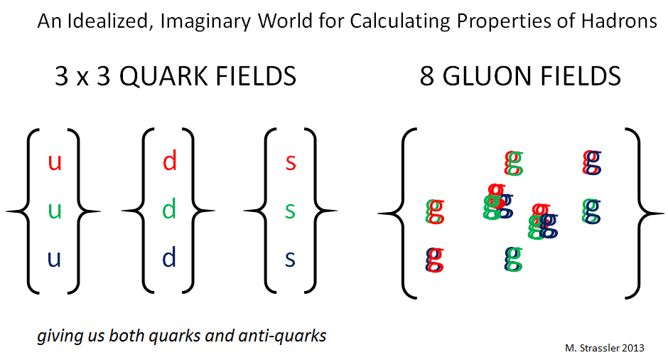
One class of methods involves directly simulating, using a computer, the behavior of the quantum field theory equations for the strong nuclear force. More precisely, we simulate in a simplified version of the real world, the imaginary world shown in Figure 1 below, where

  • the weak nuclear force and the electromagnetic force are turned off,
  • the electron, muon, tau, neutrinos, W, Z and Higgs particles are ignored
  • the three heavier types of quarks are also ignored

(See Figure 4 of Part 4 for more details.)  This makes the calculations a lot simpler.  And their results allow us, for instance, to understand why quarks and anti-quarks and gluons form the more complex particles called hadrons, of which protons and neutrons are just a couple of examples. Unfortunately, computer simulations still are nowhere near powerful enough for the calculation of some of the most interesting processes in nature… and won’t be for a long time.

Fig 1:
Fig 1: The idealized, imaginary world whose quantum field theory is used to make computer simulations of the real-world strong-nuclear force.

Another method I mentioned involves the use of an effective quantum field theory which describes the “objects” that the original theory produces at low energy. But that only works if you know what those objects are; in the real world [and the similar imaginary world of Figure 1] we know from experiment that those objects are pions and other low-mass hadrons, but generally we don’t know what they are.

This brings us to today’s story.  Our success with the Standard Model might give you the impression that we basically understand quantum field theory and how to make predictions using it, with a few exceptions. But this would be far, far from the truth. As far as we can tell, much (if not most) of quantum field theory remains deeply mysterious. (more…)

Picture of POSTED BY Matt Strassler

POSTED BY Matt Strassler

ON November 6, 2013

[This is part 5 of a series, which begins here.]

In a previous post, I told you about how physicists use computers to study how the strong nuclear force combines certain elementary particles — specifically quarks and anti-quarks and gluons — into hadrons, such as protons and neutrons and pions.  Computers can also be used to study certain other phenomena that, because they involve the strong nuclear force where it is truly “strong” [in the technical sense described here], can’t be studied using simpler methods of successive approximation. While computers aren’t a panacea, they do allow some important and difficult questions about the strong nuclear force to be answered with precision.

To do these calculations, physicists study an imaginary world, as I described;

  • all forces except the strong nuclear force are ignored, and
  • all particles are forgotten except the gluons and the up, down and strange quarks (and their anti-quarks).
  • On top of this, the up, down and strange quark masses are typically changed. They are taken larger, which makes the calculations easier, and then gradually reduced towards their small values in the real world.

The Notion of “Effective” Quantum Field Theories

There’s one more interesting method for understanding the strong nuclear force that I haven’t mentioned yet, and it too involves changing the quark masses — making them smaller, rather than larger! And weirdly, this doesn’t involve the equations of the quantum field theory for the quarks, antiquarks and gluons at all. It involves a different quantum field theory altogether — one which says nothing about the quarks and gluons, but instead describes the physics of the hadrons themselves. More precisely, its equations are useful for making predictions about the hadrons of lowest mass — called pions, kaons and etas — and it works for processes

  • with rather low energy — too low to affect the behavior of the quarks and anti-quarks and gluons inside the pions — and
  • at rather long distance — too long to detect that the pions have a lot of internal structure.

This includes some of the phenomena involved in the physics of atomic nuclei, the next level up in the structure of matter (quarks/gluons → protons/neutrons → nuclei → atoms → molecules). (more…)

Picture of POSTED BY Matt Strassler

POSTED BY Matt Strassler

ON October 28, 2013

In sports, as in science, there are two very different types of heroes.  There are the giants who lead the their teams and their sport, winning championships and accolades, for years, and whose fame lives on for decades: the Michael Jordans, the Peles, the Lou Gherigs, the Joe Montanas. And then there are the unlikely heroes, the ones who just happen to have a really good day at a really opportune time; the substitute player who comes on the field for an injured teammate and scores the winning goal in a championship; the fellow who never hits a home run except on the day it counts; the mediocre receiver who turns a short pass into a long touchdown during the Super Bowl.  We celebrate both types, in awe of the great ones, and in amused pleasure at the inspiring stories of the unlikely ones.

In science we have giants like Newton, Darwin, Boyle, Galileo… The last few decades of particle physics brought us a few, such as Richard Feynman and Ken Wilson, and others we’ll meet today.  Many of these giants received Nobel Prizes.   But then we have the gentlemen behind what is commonly known as the Higgs particle — the little ripple in the Higgs field, a special field whose presence and properties assure that many of the elementary particles of nature have mass, and without which ordinary matter, and we ourselves, could not exist.  Following discovery of this particle last year, and confirmation that it is indeed a Higgs particle, two of them, Francois Englert and Peter Higgs, have been awarded the 2013 Nobel Prize in physics.  Had he lived to see the day, Robert Brout would have been the third.

My articles Why The Higgs Particle Matters and The Higgs FAQ 2.0; the particles of nature and what they would be like if the Higgs field were turned off; link to video of my public talk entitled The Quest for the Higgs Boson; post about why Higgs et al. didn’t win the 2012 Nobel prize, and about how physicists became convinced since then that the newly discovered particle is really a Higgs particle;

The paper written by Brout and Englert; the two papers written by Higgs; the paper written by Gerald Guralnik, Tom Kibble and Carl Hagen; these tiny little documents, a grand total of five and one half printed pages — these were game-winning singles in the bottom of the 9th, soft goals scored with a minute to play, Hail-Mary passes by backup quarterbacks — crucial turning-point papers written by people you would not necessarily have expected to find at the center of things.  Brout, Englert, Higgs, Guralnik, Kibble and Hagen are (or rather, in Brout’s case, sadly, were) very fine scientists, intelligent and creative and clever, and their papers, written in 1964 when they were young men, are imperfect but pretty gems.  They were lucky: very smart but not extraordinary physicists who just happened to write the right paper at the right time. In each case, they did so

History in general, and history of science in particular, is always vastly more complex than the simple stories we tell ourselves and our descendants.  Making history understandable in a few pages always requires erasing complexities and subtleties that are crucial for making sense of the past.  Today, all across the press, there are articles explaining incorrectly what Higgs and the others did and why they did it and what it meant at the time and what it means now.  I am afraid I have a few over-simplified articles of my own. But today I’d like to give you a little sense of the complexities, to the extent that I, who wasn’t even alive at the time, can understand them.  And also, I want to convey a few important lessons that I think the Hi(gg)story can teach both experts and non-experts.  Here are a couple to think about as you read:

1. It is important for theoretical physicists, and others who make mathematical equations that might describe the world, to study and learn from imaginary worlds, especially simple ones.  That is because

  • 1a. one can often infer general lessons more easily from simple worlds than from the (often more complicated) real one, and
  • 1b. sometimes an aspect of an imaginary world will turn out to be more real than you expected!

2. One must not assume that research motivated by a particular goal depends upon the achievement of that goal; even if the original goal proves illusory, the results of the research may prove useful or even essential in a completely different arena.

My summary today is based on a reading of the papers themselves, on comments by John Iliopoulos, and on a conversation with Englert, and on reading and hearing Higgs’ own description of the episode.

The story is incompletely but perhaps usefully illustrated in the figure below, which shows a cartoon of how four important scientific stories of the late 1950s and early 1960s came together. They are:

  1. How do superconductors (materials that carry electricity without generating heat) really work?
  2. How does the proton get its mass, and why are pions (the lightest hadrons) so much lighter than protons?
  3. Why do hadrons behave the way they do; specifically, as suggested by J.J. Sakurai (who died rather young, and after whom a famous prize is named), why are there photon-like hadrons, called rho mesons, that have mass?
  4. How does the weak nuclear force work?  Specifically, as suggested by Schwinger and developed further by his student Glashow, might it involve photon-like particles (now called W and Z) with mass?

These four questions converged on a question of principle: “how can mass be given to particles?”, and the first, third and fourth were all related to the specific question of “how can mass be given to photon-like particles?’’  This is where the story really begins.  [Almost everyone in the story is a giant with a Nobel Prize, indicated with a parenthetic (NPyear).]

My best attempt at a cartoon history...
My best attempt at a cartoon history…

In 1962, Philip Anderson (NP1977), an expert on (among other things) superconductors, responded to suggestions and questions of Julian Schwinger (NP1965) on the topic of photon-like particles with mass, pointing out that a photon actually gets a mass inside a superconductor, due to what we today would identify as a sort of “Higgs-type’’ field made from pairs of electrons.  And he speculated, without showing it mathematically, that very similar ideas could apply to empty space, where Einstein’s relativity principles hold true, and that this could allow elementary photon-like particles in empty space to have mass, if in fact there were a kind of Higgs-type field in empty space.

In all its essential elements, he had the right idea.  But since he didn’t put math behind his speculation, not everyone believed him.  In fact, in 1964 Walter Gilbert (NP1980 for chemistry, due to work relevant in molecular biology — how’s that for a twist?) even gave a proof that Anderson’s idea couldn’t work in empty space!

But Higgs immediately responded, arguing that Gilbert’s proof had an important loophole, and that photon-like particles could indeed get a mass in empty space.

Meanwhile, about a month earlier than Higgs, and not specifically responding to Anderson and Gilbert, Brout and Englert wrote a paper showing how to get mass for photon-like particles in empty space. They showed this in several types of imaginary worlds, using techniques that were different from Higgs’ and were correct though perhaps not entirely complete.

A second paper by Higgs, written before he was aware of Brout and Englert’s work, gave a simple example, again in an imaginary world, that made all of this much easier to understand… though his example wasn’t perhaps entirely convincing, because he didn’t show much detail.  His paper was followed by important theoretical clarifications from Guralnik, Hagen and Kibble that assured that the Brout-Englert and Higgs papers were actually right.  The combination of these papers settled the issue, from our modern perspective.

And in the middle of this, as an afterthought added to his second paper only after it was rejected by a journal, Higgs was the first person to mention something that was, for him and the others, almost beside the point — that in the Anderson-Brout-Englert-Higgs-Guralnik-Hagen-Kibble story for how photon-like particles get a mass, there will also  generally be a spin-zero particle with a mass: a ripple in the Higgs-type field, which today we call a Higgs-type particle.  Not that he said very much!   He noted that spin-one (i.e. photon-like) and spin-zero particles would come in unusual combinations.  (You have to be an expert to even figure out why that counts as predicting a Higgs-type particle!)  Also he wrote the equation that describes how and why the Higgs-type particle arises, and noted how to calculate the particle’s mass from other quantities.  But that was it.  There was nothing about how the particle would behave, or how to discover it in the imaginary worlds that he was considering;  direct application to experiment, even in an imaginary world, wasn’t his priority in these papers.

Equation (2b) is the first time the Higgs particle explicitly appears in its modern form
In his second paper, Higgs considers a simple imaginary world with just a photon-like particle and a Higgs-type field.  Equation 2b is the first place the Higgs-type particle explicitly appears in the context of giving photon-like particles a mass (equation 2c).  From Physical Review Letters, Volume 13, page 508

About the “Higgs-type” particle, Anderson says nothing; Brout and Englert say nothing; Guralnik et al. say something very brief that’s irrelevant in any imaginable real-world application.  Why the silence?  Perhaps because it was too obvious to be worth mentioning?  When what you’re doing is pointing out something really “important’’ — that photon-like particles can have a mass after all — the spin-zero particle’s existence is so obvious but so irrelevant to your goal that it hardly deserves comment.  And that’s indeed why Higgs added it only as an afterthought, to make the paper a bit less abstract and a bit easier for  a journal to publish.  None of them could have imagined the hoopla and public excitement that, five decades later, would surround the attempt to discover a particle of this type, whose specific form in the real world none of them wrote down.

In the minds of these authors, any near-term application of their ideas would probably be to hadrons, perhaps specifically Sakurai’s theory of hadrons, which in 1960 predicted the “rho mesons”, which are photon-like hadrons with mass, and had been discovered in 1961.  Anderson, Brout-Englert and Higgs specifically mention hadrons at certain moments. But none of them actually considered the real hadrons of nature, as they were just trying to make points of principle; and in any case, the ideas that they developed did not apply to hadrons at all.  (Well, actually, that’s not quite true, but the connection is too roundabout to discuss here.)  Sakurai’s ideas had an element of truth, but fundamentally led to a dead end.  The rho mesons get their mass in another way.

Meanwhile, none of these people wrote down anything resembling the Higgs field which we know today — the one that is crucial for our very existence — so they certainly didn’t directly predict the Higgs particle that was discovered in 2012.   It was Steven Weinberg (NP1979) in 1967, and Abdus Salam (NP1979) in 1968, who did that.  (And it was Weinberg who stuck Higgs’ name on the field and particle, so that everyone else was forgotten.) These giants combined

  • the ideas of Higgs and the others about how to give mass to photon-like particles using a Higgs-type field, with its Higgs-type particle as a consequence…
  • …with the 1960 work of Sheldon Glashow (NP1979), Schwinger’s student, who like Schwinger proposed the weak nuclear force was due to photon-like particles with mass,…
  • …and with the 1960-1961 work of Murray Gell-Man (NP1969) and Maurice Levy and of Yoichiro Nambu (NP2008) and Giovanni Jona-Lasinio, who showed how proton-like or electron-like particles could get mass from what we’d now call Higgs-type fields.

This combination gave the first modern quantum field theory of particle physics: a set of equations that describe the weak nuclear and electromagnetic forces, and show how the Higgs field can give the W and Z particles and the electron their masses. It is the primitive core of what today we call the Standard Model of particle physics.  Not that anyone took this theory seriously, even Weinberg.  Most people thought quantum field theories of this type were mathematically inconsistent — until in 1971 Gerard ‘t Hooft (NP1999) proved they were consistent after all.

The Hi(gg)story is populated with giants.  I’m afraid my attempt to tell the story has giant holes to match.  But as far as the Higgs particle that was discovered last year at the Large Hadron Collider, the unlikely heroes of the story are the relatively ordinary scientists who slipped in between the giants and actually scored the goals.

Picture of POSTED BY Matt Strassler

POSTED BY Matt Strassler

ON October 8, 2013

This year’s Nobel Prize, presumably to be given for the prediction of the particle known today as the “Higgs boson”, will be awarded next week.  But in the meantime, the American Physical Society has made a large number of awards.  A few of them are to people whose work I know about, so I thought I’d tell you just a little about them.

The J. J. Sakurai prize went to Professors Zvi Bern, Lance Dixon and David Kosower, for the work that I have already described on this website here and here.  Dixon, a wide-ranging expert in particle physics, quantum field theory and string theory, was a young professor at the Stanford Linear Accelerator Center when I was a Stanford graduate student.  He taught an excellent course on string theory, and provided a lot of scientific advice and insight outside the classroom.  Bern and Kosower were young scientists using string theory to learn about how to do computations in quantum field theory, and their surprising results formed the starting point for my Ph. D. thesis (which has their names in its title.)   The range of their work is hard to describe in a paragraph, but let’s just say that no one is surprised that they were awarded a prize of this magnitude.

The Dannie Heineman Prize for Mathematical Physics was awarded to my former colleague Greg Moore, a professor at Rutgers University.  “For eminent contributions to mathematical physics with a wide influence in many fields, ranging from string theory to supersymmetric gauge theory, conformal field theory, condensed matter physics and four-manifold theory.”  Allow me to translate:

  • string theory: you’ve heard about it, probably
  • supersymmetric gauge theory: quantum field theories with supersymmetry, which I’ll be writing about soon
  • conformal field theory: basically, quantum field theories that are scale invariant
  • condensed matter physics: the study of solids and liquids and their mechanical and electrical properties, and lots of other things too, in which quantum field theory is sometimes a useful tool
  • four-manifold theory: the mathematics of spaces which have four-spatial dimensions, or three-spatial dimensions and one-time dimension.  These spaces are very interesting to mathematicians, and also, they’re interesting because we live in one.

This is not the complete range of Moore’s work by any means.  Unfortunately this website doesn’t yet have pages that can put his work in proper context, but perhaps I’ll return to it later.  But again, no surprise here to see Moore’s name on this award.

The Tom W. Bonner Prize in Nuclear Physics was awarded to experimental physicist William A. Zajc, currently chairman of the Columbia University physics department.  Zajc has been heavily involved in one of the most surprising discoveries of the past fifteen years: that a hot dense fireball of quarks, anti-quarks and gluons (produced in the collision of two relatively large atomic nuclei) behaves in a very unexpected way, more like a very low viscosity liquid rather like than a gas.  I’ve known him partly because of his interest in the attempts to apply string theory to certain quantum field theories that are perhaps relevant in the modeling of this novel physical system… something I’ll also probably be writing about in the relatively near future.

And the W.K.H. Panofsky Prize in Experimental Particle Physics went to Kam-Biu Luk (Berkeley) and Yifang Wang (Director of China’s Institute of High Energy Physics): For their leadership of the Daya Bay experiment, which produced the first definitive measurement of the theta-13 angle of the neutrino mixing matrix.  For the same experiment, the Henry Primakoff Award for Early-Career Particle Physics went to Daniel A. Dwyer of Lawrence Berkeley Laboratory.  I wrote about the Daya Bay measurement here; their result is one of the major measurements in particle physics in the past few years.

I wish I knew more about the other recipients outside my areas of expertise, but other bloggers will have to cover those stories.

Anyway, no surprises, but some very deserving scientists.  Let’s see if next Tuesday brings the same result.

Picture of POSTED BY Matt Strassler

POSTED BY Matt Strassler

ON October 3, 2013

[This is the third post in a series; here’s #1 and #2.]

The quantum field theory that we use to describe the known particles and forces is called the “Standard Model”, whose structure is shown schematically in Figure 1. It involves an interweaving of three quantum field theories — one for the electromagnetic force, one for the weak nuclear force, and one for the strong nuclear force — into a single more complex quantum field theory.

SM_Interactions
Fig. 1: The three non-gravitational forces, in the colored boxes, affect different combinations of the known apparently-elementary particles. For more details see http://profmattstrassler.com/articles-and-posts/particle-physics-basics/the-known-apparently-elementary-particles/

We particle physicists are extremely fortunate that this particular quantum field theory is just one step more complicated than the very simplest quantum field theories. If this hadn’t been the case, we might still be trying to figure out how it works, and we wouldn’t be able to make detailed and precise predictions for how the known elementary particles will behave in our experiments, such as those at the Large Hadron Collider [LHC].

In order to make predictions for processes that we can measure at the LHC, using the equations of the Standard Model, we employ a method of successive approximation (with the jargon name “method of perturbations”, or “perturbation `theory’ ”). It’s a very common method in math and science, in which

  • we make an initial rough estimate,
  • and then correct the estimate,
  • and then correct the correction,
  • etc.,

until we have a prediction that is precise enough for our needs.

What are those needs? Well, the precision of any measurement, in any context, is always limited by having

  • a finite amount of data (so small statistical flukes are common)
  • imperfect equipment (so small mistakes are inevitable).

What we need, for each measurement, is a prediction a little more precise than the measurement will be, but not much more so. In the difficult environment of the LHC, where measurements are really hard, we often need only the first correction to the original estimate; sometimes we need the second (see Figure 2).

Fig. 2: LONLONNLO
Fig. 2: Top quark/anti-quark pair production rate as a function of the energy of the LHC collisions, as measured by the LHC experiments ATLAS and CMS, and compared with the prediction within the Standard Model.  The measurements are the colored points, with bars indicating their uncertainties.  The prediction is given by the colored bands — purple for the initial estimate, red after the first correction, grey after the second correction — whose widths indicate how uncertain the prediction is at each stage.  The grey band is precise enough to be useful, because its uncertainties are comparable to those of the data.  And the data and Standard Model prediction agree!

Until recently the calculations were done by starting with Feynman’s famous diagrams, but the diagrams are not as efficient as one would like, and new techniques have made them mostly obsolete for really hard calculations.

The method of successive approximation works as long as all the forces involved are rather “weak”, in a technical sense. Now this notion of “weak” is complicated enough (and important enough) that I wrote a whole article on it, so those who really want to understand this should read that article. The brief summary suitable for today is this: suppose you took two particles that are attracted to each other by a force, and allowed them to glom together, like an electron and a proton, to form an atom-like object.  Then if the relative velocity of the two particles is small compared to the speed of light, the force is weak. The stronger the force, the faster the particles will move around inside their “atom”.  (For more details see this article. )

For a weak force, the method of successive approximation is very useful, because the correction to the initial estimate is small, and the correction to the correction is smaller, and the correction to the correction to the correction is even smaller. So for a weak force, the first or second correction is usually enough; one doesn’t have to calculate forever in order to get a sufficiently precise prediction. The “stronger” the force, in this technical sense, the harder you have to work to get a precise prediction, because the corrections to your estimate are larger.

If a force is truly strong, though, everything breaks down. In that case, the correction to the estimate is as big as the estimate, and the next correction is again just as big, so no method of successive approximation will get you close to the answer. In short, for truly strong forces, you need a completely different approach if you are to make predictions.

In the Standard Model, the electromagnetic force and the weak nuclear force are “weak” in all contexts. However, the strong nuclear force is (technically) “strong” for any processes that involve distances comparable to or larger than a proton‘s size (about 100,000 times smaller than an atom) or energies comparable to or smaller than a proton’s mass-energy (about 1 GeV). For such processes, successive approximation does not work at all; it can’t be used to calculate a proton’s size or mass or internal structure. In fact the first step in that method would estimate that quarks and anti-quarks and gluons are free to roam independently and the proton should not exist at all… which is so obviously completely wrong that no method of correcting it will ever give the right answer.  I’ll get back to how we show protons are predicted by these equations, using big computers, in a later post.

But there’s a remarkable fact about the strong nuclear force. As I said, at distances the size of a proton or larger, the strong nuclear force is so strong that successive approximation doesn’t work. Yet, at distances shorter than this, the force actually becomes “weak”, in the technical sense, and successive approximation does work there.

Let me make sure this is absolutely clear, because the difference between what we think of colloquially as “weak” is different from “weak” in the sense I’m using it here.  Suppose you put two quarks very close together, at a distance r closer together than the radius R of a proton.  In Figure 3 I’ve plotted how big the strong nuclear force (purple) and the electromagnetic force (blue) would be between two quarks, as a function of the distance between them. Notice both forces are very strong (colloquially) at short distances (r << R), but (I assert) both forces are weak (technically) there.  The electromagnetic force is much the weaker of the two, which is why its curve is lower in the plot.  

Now if you move the two quarks apart a bit (increasing r, but still with r << R), both forces become smaller; in fact both decrease almost like 1/r², which would be your first, naive estimate, same as in your high school science class. If this naive estimate were correct, both forces would maintain the same strength (technically) at all distances r.  

But this isn’t quite right.  Since the 1950s, it was well-known that the correction to this estimate (using successive approximation methods) is to make the electromagnetic force decrease just a little faster than that; it becomes a tiny bit weaker (technically) at longer distances.  In the 60s, that’s what most people thought any force described by quantum field theory would do. But they were wrong.  In 1973, David Politzer, and David Gross and Frank Wilczek, showed that for the quantum field theory of quarks and gluons, the correction to the naive estimate goes the other direction; it makes the force decrease just a little more slowly than 1/r². [Gerard ‘t Hooft had also calculated this, but apparently without fully recognizing its importance…?] It is the small, accumulating excess above the naive estimate — the gradual deviation of the purple curve from its naive 1/r² form — that leads us to say that this force becomes technically “stronger” and “stronger” at larger distances. Once the distance r becomes comparable to a proton’s size R, the force becomes so “strong” that successive approximation methods fail.  As shown in the figure, we have some evidence that the force becomes constant for r >> R, independent of distance.  It is this effect that, as we’ll see next time, is responsible for the existence of protons and neutrons, and therefore of all ordinary matter.

Fig. 3: How the electromagnetic force (blue) and the strong nuclear force (purple) vary as a function of the distance r between two particles that feel the corresponding force. The horizontal axis shows r in units of the confinement scale R; the vertical axis shows the force in units of the minimum strength of the strong nuclear force, which it exerts for r > R.
Fig. 3: How the electromagnetic force (blue) and the strong nuclear force (purple) vary as a function of the distance r between two quarks. The horizontal axis shows r in units of the proton’s radius R; the vertical axis shows the force in units of the constant value that the strong nuclear force takes for r >> R.  Both forces are “weak” at short distances, but the strong nuclear force becomes “strong” once r is comparable to, or larger than, R.

So: at very short distances and high energies, the strong nuclear force is a somewhat “weak” force, stronger still than the electromagnetic and weak nuclear forces, but similar to them.  And therefore, successive approximation can tell you what happens when a quark inside one speeding proton hits a quark in a proton speeding the other direction, as long as the quarks collide with energy far more than 1 GeV. If this weren’t true, we could make scarcely any predictions at the LHC, and at similar proton-proton and proton-antiproton colliders! (We do also need to know about the proton’s structure, but we don’t calculate that: we simply measure it in other experiments.)  In particular, we would never have been able to calculate how often we should be making top quarks, as in Figure 2.  And we would not have been able to calculate what the Standard Model, or any other quantum field theory, predicts for the rate at which Higgs particles are produced, so we’d never have been sure that the LHC would either find or exclude the Standard Model Higgs particle. Fortunately, it is true, and that is why precise predictions can be made, for so many processes, at the LHC.  And the success of those and other predictions underlies our confidence that the Standard Model correctly describes most of what we know about particle physics.

But still, the equations of the strong nuclear force have only quarks and anti-quarks and gluons in them — no protons, neutrons, or other hadrons.  Our understanding of the real world would certainly be incomplete if we didn’t know why there are protons.  Well, it turns out that if we want to know whether protons and neutrons and other hadrons are actually predicted by the strong nuclear force’s equations, we have to test this notion using big computers. And that’s tricky, even trickier than you might guess.

Continued here


Picture of POSTED BY Matt Strassler

POSTED BY Matt Strassler

ON October 1, 2013

I spent the last two days at an extraordinary conference, “Dreams of Earth and Sky”, celebrating the life and career of an extraordinary man, one of the many fascinating scientists whom I have had the good fortune to meet. I am referring to Freeman Dyson, professor at the Institute for Advanced Study (IAS), whose career has spanned so many subfields of science and beyond that the two-day conference simply wasn’t able to represent them all.

DysonPhoto

The event, held on the campus of the IAS, marked Dyson’s 90th year on the planet and his 60th year as a professor. (In fact his first stay at the IAS was a few years even earlier than that.) The IAS was then still a young institution; Albert Einstein, John Von Neumann, Kurt Gödel and J. Robert Oppenheimer were among the faculty. Dyson’s most famous work in my own field was on the foundations of the quantum field theory of the electromagnetic force, “quantum electrodynamics”, or “QED”.  His work helped explain its mathematical underpinnings and clarify how it worked, and so impressed Oppenheimer that he got Dyson a faculty position at the IAS. This work was done at a very young age.  By the time I arrived to work at the IAS in 1996, Dyson had officially retired, but was often in his office and involved in lunchtime conversations, mostly with the astronomers and astrophysicists, which is where a lot of his late career work has been centered.

Retirement certainly hasn’t stopped Dyson’s activity. His mind seems to be ageless; he is spry, attentive, sharp, and still doing science and writing about it and other topics. When I went up to congratulate him, I was surprised that he not only remembered who I was, he remembered what I had been working on in 1992, when, as an unknown graduate student on the other coast, I had sent him a paper I had written.

By the way, it’s somewhat bizarre that Dyson never won a Nobel Prize.  Arguably it is part of the nature of the awarding process, which typically rewards a specific, deep line of research, and not a polymath whose contributions are spread widely.  Just goes to show that you have to look at the content of a person’s life and work, not the prizes that someone thought fit to award to him or her.  Still, he has his share: Dannie Heineman Prize for Mathematical Physics 1965; German Physical Society, Max Planck Medal 1969; Harvey Prize 1977; Wolf Foundation Prize in Physics 1981; American Association of Physics Teachers, Oersted Medal 1991; Enrico Fermi Award 1995; Templeton Prize for Progress in Religion 2000; Henri Poincaré Prize 2012.

The thirteen talks and several brief comments given at the conference, all of which in one way or another related to Dyson’s work, were organized into sessions on mathematics, on physics and chemistry, on astronomy and astrobiology, and on public affairs. All of the speakers were eminent in their fields, and I encourage you to explore their websites and writings, some of which were controversial, all of which were interesting. For non-scientists, I especially recommend Stanford Professor Emeritus Sid Drell’s extremely interesting talk about nuclear disarmament (which he’s been working towards for decades), and a thought-provoking if disconcertingly slick presentation by Dr. Amory Lovins of the Rocky Mountain Institute on what he sees as a completely realistic effort, already underway, to wean the United States of its addiction to oil — with no net cost. Those with a small to moderate amount of scientific background may especially enjoy MIT Professor Sara Seager’s work on efforts to discover and study planets beyond our own solar system, Texas Professor Bill Press’s proposal for how to rethink the process of drug trials and approvals in the age of electronic patient records, Sir Martin Rees’s views on the state of our understanding of the universe, and Caltech’s Joseph Kirschvink’s contention that scientific evidence tends to favor the notion that life on this planet most likely started on Mars.

But really, if you haven’t heard about all the different things Freeman Dyson has done, or read any of his writings, you should not miss the opportunity. Start here and here, and enjoy!

Many happy returns, Professor Dyson; you have been an inspiration and a role model for several generations of young scientists, and may you have many more happy and healthy years to come!

Picture of POSTED BY Matt Strassler

POSTED BY Matt Strassler

ON September 29, 2013

[This post is a continuation of this one from Monday]

Coming to Terms

Before we continue, a little terminology — trivial, yet crucial and slightly subtle.

Think about the distinction between the words “humanity” and “a human” and “humans”; or “higher education”, “university” and “universities”; or “royalty”, “king” and “kings”. In each case, the three words refer to the general case, the specific case, and a group of specific cases.  Sometimes you even have to use context to figure out whether you’re dealing with the general case or a group, because “humans” or “kings” is sometimes used in place of “humanity” or “royalty”.

In a similar way:

  • The words “quantum field theory” (with no word in front) refers to the general case: the general type of equations that we use for particle physics and many other fields of study.
  • The words “a quantum field theory” refers to a particular case; an example of a set of equations drawn from the general case called “quantum field theory”.
  • The words “quantum field theories” refers to a group of particular cases: a set of examples, perhaps ones that share something in common. We might talk about “some quantum field theories”, or “all quantum field theories”, or “a few quantum field theories”.

Before I go on, I should probably point out that string theory/M theory is different, for a weird (and perhaps temporary) reason — it appears (currently) that there’s only one such theory that has fully consistent mathematics and contains a quantum version of Einstein’s theory of gravity.  That was figured out in the 1990s.

However, in that theory you need another, similar distinction. Let me postpone a proper definition until later, but roughly, a “string vacuum” is a particular way that string/M theory could manifest itself in a universe; if you changed the string vacuum that we’re in (says string theory), we’d end up with different particles and forces and somewhat different laws governing those particles and forces. Many such vacua would have particles and forces described by a quantum field theory, along with Einstein’s gravity; many (perhaps most) other vacua might not have this property.  And so, as before, we need to distinguish “string vacua in general”, “a string vacuum”, and “string vacua”, plural.

Now it’s time to talk about quantum field theory — the general case — in more detail.

Quantum Field Theory and Its Predictions

Does quantum field theory as a whole predict anything? In short, if you knew a universe had physics described by a quantum field theory, but you didn’t know which particular quantum field theory, what could you predict?

The answer is: almost nothing.

If you’ve been following this blog with care, or have read some books or articles about particle physics, you might well think: quantum field theories have fields; and fields have particles; so here’s a prediction: there should be some particles of some type.

Nope.  You’ve learned your lesson well — everything I’ve told you on this website suggests that it is true — but the conclusion is false. I’ve been white-lying to you this whole time, and I have to apologize for that. Quantum fields do often have particles. But many quantum field theories are scale-invariant. A scale-invariant thing looks and behaves more or less the same in a microscope no matter how strong a lens you use. The wikipedia article on scale invariance actually has a nice animation of a scale-invariant process. Another example of something scale-invariant is a fractal. And in a scale-invariant quantum field theory (except for one in which there are no forces at all), there are no particles. I’ve told you that particles are well-behaved ripples in fields… well, it’s true, but in a scale-invariant quantum field theory with at least one force, any such ripples die away and turn into several ripples, which die away and turn into several ripples, which die away and turn into several ripples, which die away and turn into several ripples, which…

Wiener_process_animated
Click here to see an animation of a scale-invariant process, called the Wiener process. Animation from Wikimedia Commons (author Cyp). For more information, see http://en.wikipedia.org/wiki/File:Wiener_process_animated.gif

In short, no particles. This has been known for many decades (I’m actually not sure how far it goes back in the form I just described.) We observe this behavior in experiments — not in particle physics, where it isn’t relevant (at least currently), but in many solids, liquids, electrical conductors, magnets etc. that are undergoing “phase transitions”, such as melting, or spontaneous magnetization. In some cases we can also calculate this behavior, exactly or approximately. In some cases we can see this behavior emerge in computer simulations of real or imaginary materials. So we know there are many quantum field theories that don’t have particles.

[This might make you wonder if there are string/M theory vacua that don’t have strings. Good thinking… though actually there are other, unrelated ways to end up without strings… more on this later in the month.]

But If There Are Particles… A Prediction!

But here’s something important that we can predict. If we are studying a quantum field theory that does have particles (now we are talking not about all quantum field theories, but an interesting subset of them) then

  • the particles will come in types (in our world, electrons are examples of a type of particle, Higgs particles are an example of another, etc.); and
  • two particles of the same type will be identical in all their intrinsic properties. They will have the same electric charge, spin, mass [i.e. rest mass] etc.; if somebody swaps one for another, you won’t be able to tell the difference.  (In our world, all electrons are identical.)
  • Furthermore, in a world with three (or more) spatial dimensions in which Einstein’s special relativity is true, then particles of each type will be either fermions or bosons. (The Pauli Exclusion Principle, which determines all of atomic physics and chemistry, is a consequence of the facts that all electrons are identical and that electrons are fermions.)

Again, these are general prediction, not of quantum field theory as a whole, but of the subset of quantum field theories that have particles in the first place.  The Standard Model, the quantum field theory that seems to describe much of our world very well so far, is an example of one that has particles.

That these are the most important predictions of quantum field theory with particles was pointed out to me, when I was just out of graduate school 20 years ago, by none other than Freeman Dyson, who helped develop quantum field theory back in its infancy.

Moving Toward Particular Quantum Field Theories

Now, what about specific quantum field theories. What can we predict about them?

The answer, hardly surprising, is: it depends.

  • In some quantum field theories, we can predict an enormous amount, by doing some straightforward type of calculation.
  • In others, brute-force computer simulation of the quantum fields makes it possible to study the particles and forces described by that quantum field theory, and allows us to make some predictions.
  • In some quantum field theories, we can predict a smattering of things very well, using fancy math methods (for example, using fancy geometry, or supersymmetry, or string theory).
  • In still others… unfortunately, many of the most interesting… we have absolutely no idea what’s going on.  Sometimes we have the equations we’re supposed to use, but none of our methods for calculation work for those equations.  Occasionally we can make a good guess, but we can’t always check it.
  • In yet others, we don’t even know what the equations are that we should use to start studying them.  In fact, the existence of some of these theories was, until relatively recently, unknown. We didn’t even suspect they existed.  Maybe there are even more that we still don’t know about.

I’ll start describing these categories of quantum field theories in my ensuing posts.  Fortunately for particle physicists, the Standard Model is mostly in the first category, with a little leakage into the second.

The Standard Model: A Quantum Field Theory Of Particular Significance

Continued HERE.

Picture of POSTED BY Matt Strassler

POSTED BY Matt Strassler

ON September 24, 2013

One of the important lessons of last Tuesday’s debate about string theory is that if I’m going to talk about theories that do or don’t predict things, I’d better be very clear about

  • what’s a theory?
  • what’s a scientific theory expected to do?
  • what’s a prediction?

On Thursday I asked my readers if they felt misled by Tuesday’s article. Most didn’t feel that way (I’m gratified), but if you’re a good scientist you focus attention on the negative feedback you receive, because that’s where you are most likely to learn something. And you also look for negative signs in the positive feedback. So thank you, especially those who were critical yet reasonable. I will respond in due course, by putting out a better, clearer article on what string theory can and cannot do, on what we know and do not know about it, a bit about its history, etc. Then I can avoid creating or contributing to confusions, such as the ones Dr. Woit expressed concerns about.

But today I want to explain why I found my conversation with Dr. Woit troubling scientifically (as opposed to pedagogically or politically). It wasn’t because I’m a string theorist — in fact, I’m not a string theorist, by anyone’s reasonable definition (except possibly Dr. Woit’s [and probably not even by his.])

I’m a quantum field theorist. Quantum field theory is the mathematical language of particle physics; quantum field theory equations are used to describe and predict the behavior of the known elementary particles and forces of nature.  Throughout my 25 year career I have mainly studied quantum field theory and some of its applications. Its applications are many. I have focused on the applications to particle physics, with some also to string theory, astronomy and cosmology, and even quantum gravity. (Other applications that I haven’t worked on include the physics of “condensed matter” — solids and liquids; magnets; electrical conductors, insulators, and superconductors; and a lot of weirder things — and phase transitions, such as the melting of a solid to a liquid, or the change of a material from magnet to a non-magnet.)

And meanwhile, while doing quantum field theory, I use every tool I can. I use fancy math. I use what I can learn from other people’s experiments, or from their big numerical simulations.  Sometimes I use string theory. Sometimes I use computers.   If loop quantum gravity were useful as a tool for quantum field theory, I’d use it. Heck, I’d use formaldehyde, bulldozers, musical instruments and/or crowds of hypnotized rats if it would help me understand quantum field theory. I’ve got a job to do, and I’m not going to stray from it just because somebody with a different job (or an axe to grind) loves or hates my tools.

The Scientific Issue

So here’s what bothers me about Dr. Woit’s argument.  First he said: “to deal with the scientific issue here and make an accurate statement, one needs to first address the following:

  1. What is a prediction?
  2. What is string theory?
  3. What are the vacuum states of string theory?“

Hard to argue with that!  [He elaborated on each of these three points, but I leave it to you to go back and read the elaboration if you like.]  And then he concludes:

“What is the difference between this situation and Quantum Field Theory? That’s pretty simple: no problems 2 and 3. And those problems are not problems of calculations being hard.”

Woit’s implication is that we do know what field theory is and we do understand the vacua of field theory… and that while prediction in field theory is merely hard in practice, we know what we are doing… and that we understand so little about string theory that prediction in string theory is impossible in principle.  This, as a quantum field theorist, I strongly disagree with.  

If you are concerned, as you should always be in these situations, that Woit’s being misquoted or quoted out of context, you can go back and reread the comment exchange to Tuesday’s post.

What bothers me about this is that this kind of sweeping statement does a disservice to both subjects: it understates what we know about string theory and overstates what we know about quantum field theory. If only quantum field theory always made it straightforward (albeit difficult) to make predictions! My job would be a lot easier, and it might even be much easier to solve some of the deepest puzzles in nature.

Also, this blanket statement leaves it completely unclear and mysterious why string theory could be such a helpful tool for a quantum field theorist like me — which is a real loss, because the usefulness of string theory for field theory is one of the most interesting aspects of both subjects.

Our understanding of quantum field theory, while perhaps no longer in its infancy, is still clearly in adolescence, at best — and it seems likely to me that we know even less than we think. And I think that many of my readers would like to hear more about this.

What I intend to do over the coming weeks, as time and news permits, is

  1. describe to you what we do and don’t know about quantum field theory
  2. describe to you what we do and don’t know about string theory
  3. explain how, over the past 20 or so years, we have used some of the things we do know about string theory to learn some things we didn’t know (and often didn’t know we didn’t know) about quantum field theory.
  4. describe how one can use quantum field theory to learn something more about string theory

I’ll do items numbers 1 and 3 carefully.  Specifically, in number 3, I will focus on predictions made for quantum field theory using string theory [and we’ll talk very carefully, at that time, about what “prediction” means.]) Both 2 and 4 are more nebulous, and I don’t work on them directly, but I think I can do a decent job on them. I’m sure my colleagues will correct me if I get any facts wrong.

What Does “Theory” Mean to a Physicist?

First, an important, fundamental question. When I say: “quantum field theory”, or “string theory”, or “theory of relativity” — well, what is a theory?

It’s not what it means in Webster’s dictionary of the English Language.  It’s not the same as a guess or a hypothesis. It’s not the opposite of a “fact”. It’s something much more powerful than either one.  And it’s certainly not what it means in various academic departments like Literature or Art or even Sociology.

I could write a whole article on this (and someday I might) but here’s the best definition I have at the moment.  Probably there are better definitions out there.  But here’s my best shot for now: in my line of research, a theory is a set of mathematical equations, along with a set of accompanying concepts, that can be used to make predictions for how physical objects will behave, on their own and in combination — and these predictions may be relevant either in the real world or in imaginary (but reasonable, imaginable) worlds.

Wait! Why are imaginary worlds important? Why focus on anything other than the real world?  How could studying imaginary worlds be “scientific”?

Because:

  • By studying imaginary particles and forces, we gain insight into the real world: which properties of our universe are true of all possible universes? which properties are common but not ubiquitous? which ones are special and unique to our own?
  • Sometimes the math that describes a specially chosen combination of particles and forces turns out to be much simpler than the mathematics that describes the particles and forces in our own universe. In an imaginary world described by these equations, it may be possible to solve problems that are too hard to solve in the real world.  And even though the lessons learned don’t apply directly to our world, they may still yield fundamental insights into how the real world works.
  • The future may surprise us. Things that are imaginary today might actually turn up, in future, in the real world. For instance: the top quark that we find in nature was imaginary for over 20 years; the Higgs particle was imaginary for almost 50; supersymmetry is still imaginary, and no one knows if it will remain so.]
  • Note Added: commenter Kent reminded me of another excellent reason, and an example of it: “Sometimes it is not possible to understand the real world until we have first understood an idealization of it. There are many examples … [including] the discovery of the laws of motion by Galileo and Newton. For hundreds of years, people followed Aristotle in believing that a moving object would return to its “natural state” of being at rest unless a force acted on it. Galileo and Newton’s breakthrough was their ability to imagine a world without friction or air resistance. Only after they understood this imaginary world could they properly understand the real one and learn that the natural state of an object is to continue moving in the same way UNLESS a force acts on it.“

Notice that this strategy is not unique to physics! Biologists who want to understand humans also study flies, mice, yeast, rabbits, monkeys, etc.. From this type of research — often much easier, cheaper and safer than direct research on humans — they can perhaps learn what is common to the biology of all primates, or of all mammals, or of all animals, and/or of all life on Earth, and perhaps also ascertain what it is that makes humans unique. Many experts on Earth’s geology and climate are fascinated by Mars, Venus, and the rocky moons of Saturn and Jupiter, whose similarities to and differences from Earth give us a perspective on what makes the Earth special, and what makes it typical. Kierkegaard, the philosopher, famously uses the technique of “what-if” stories — a story retold with slight differences and a quite different outcome — to try to tease apart the meaning of religious faith within the Abraham-and-Isaac story, in his famous work “Fear and Trembling”.

The Lesson: If you want to understand a particular case, study the general case, and other similar-but-yet-different particular cases, in order to gain the insights that the particular case, on its own, cannot easily give you.  Meanwhile, what you learn along the way may have wider implications that you did not anticipate.  In short, putting one’s imagination to work, in order to learn about the real, is a powerful, tried and true approach to theoretical physics.

Continued here…

Picture of POSTED BY Matt Strassler

POSTED BY Matt Strassler

ON September 23, 2013

Search

Buy The Book

Reading My Book?

Got a question? Ask it here.

Media Inquiries

For media inquiries, click here.