In recent talks at physics departments about my book, I have emphasized that the elementary “particles” of nature — electrons, photons, quarks and so on — are really little waves (or, to borrow a term that was suggested by Sir Arthur Eddington in the 1920s, “wavicles”.) But this notion inevitably generates confusion. That’s because of another wavy concept that arises in “quantum mechanics” —the quantum physics of the 1920s, taught to every physics student. That concept is Erwin Schrödinger’s famous “wave function”.
It’s natural to guess that wave functions and wavicles are roughly the same. In fact, however, they are generally unrelated.
Wavicles Versus Wave Functions
Before quantum physics came along, field theory was already used to predict the behavior of ordinary waves in ordinary settings. Field theory is useful for sound waves in air, seismic waves in rock, and waves on water.
Quantum field theory, the quantum physics that arose out of the 1940s and 1950s, adds something new: it tells us that waves in quantum fields are made from wavicles, the gentlest possible waves. A photon, for instance, is a wavicle of light — the dimmest possible flash of light.
By contrast, a wave function describes a system of objects operating according to quantum physics. Importantly, it’s not one wave function per object — it’s one wave function per system of interacting objects. That’s true whether the objects in the system are particles in motion, or something as simple as particles that cannot move, or something as complex as fields and their wavicles.
One of the points I like to make, to draw the distinction between these two types of waves in quantum physics, is this:
- Wavicles can hurt you.
- Wave functions cannot.
Daniel Whiteson, the well-known Large Hadron Collider physicist, podcaster and popular science writer, liked this phrasing so much that he quoted the second half on X/Twitter. Immediately there were protests. One person wrote “Everything that has ever hurt anyone was in truth a wave function.” Another posted a video of an unfortunate incident involving the collision between a baseball and a batter, and said: “the wave function of this baseball disagrees.”
It’s completely understandable why there’s widespread muddlement about this. We have two classes of waves floating around in quantum physics, and both of them are inherently confusing. My aim today is to make it clear why a wave function couldn’t hurt a fly, a cat, or even a particle.
The Basic Concepts
Wavicles, such as photons or electrons, are real objects. X-rays are a form of light, and are made of photons — wavicles of light. A strong beam of X-ray photons can hurt you. The photons travel across three-dimensional space carrying energy and momentum; they can strike your body, damage your DNA, and thereby cause you to develop cancer.
The wave function associated with the X-ray beam, however, is not an object. All it does is describe the beam and its possible futures. It tells us what the beam’s energy may be, but it doesn’t have any energy, and cannot inflict the beam’s energy on anything else. The wave function tells us where the beam may go, but itself goes nowhere. Though it describes a beam as it crosses ordinary three-dimensional space, the wave function does not itself exist in three-dimensional space.
In fact, if the X-ray beam is interacting with your body, then the X-ray beam cannot be said to have its own wave function. Instead, there is only one wave function — one that describes the beam of photons, your atoms, and the interactions between your atoms and the photons.
More generally, if a bunch of objects interact with each other,the multiple interacting objects form a single indivisible system, and a single wave function must describe it. The individual objects do not have separate wave functions.
Schrödinger’s Cat
This point is already illustrated by Schrödinger’s famous (albeit unrealistic) example of the cat in a box that is both dead and alive. The box contains a radioactive atom which will, via a quantum process, eventually “decay” [i.e. transform itself into a new type of atom, releasing a subatomic particle in the process], but may or may not have done so yet. If and when the atom does decay, it triggers the poisoning of the cat. The cat’s survival or demise thus depends on a quantum effect, and it becomes a party to a quantum phenomenon.
It would be a mistake to say that “the atom has a wave function” (or even worse, that “the atom is a wave function”) and that this wave function can kill the cat. To do so would miss Schrödinger’s point. Instead, the wave function includes the atom, the killing device, and the cat.
Initially, when the box is closed, the three are independent of one another, and so they have a relatively simple wave function which one may crudely sketch as
- Wave Function = (atom undecayed) x (device off) x (cat alive)
This wave function represents our certainty that the atom has not yet decayed, the murder weapon has not been triggered, and the cat is still alive.
But this initial wave function immediately begins evolving into a more complicated form, one which depends on two time-varying complex numbers C and D, with |C|2 + |D|2 = 1:
- Wave Function = C(t) x (atom undecayed) x (device off) x (cat alive) + D(t) x (atom decayed) x (device on) x (cat dead)
The wave function is now a sum of two “branches” which describe two distinct possibilities, and assigns them probabilities |C|2 and |D|2, the former gradually decreasing and the latter gradually increasing. [Note these two branches are added together in the wave function; its branches cannot be rearranged into wave functions for the atom, device and cat separately, nor can the two branches ever be separated from one another.]
In no sense has the wave function killed the cat; in one of its branches the cat is dead, but the other branch describes a live cat. And in no sense did the “wave function of the atom” or “of the device” kill the cat, because no such wave functions are well-defined in this interacting system.
A More Explicit Example
Let’s now look at an example, similar to the cat but more concrete, and easier to think about and draw.
Let’s take two particles [not wavicles] A and B. These particles travel only in a one-dimensional line, instead of in three-dimensional space.
Initially, particle B is roughly stationary and particle A comes flying toward it. There are two possible outcomes.
- There is a 30% probability that A passes right by B without affecting it, in which case B simply says “hi” as A goes by.
- There is a 70% probability that A strikes B head-on and bounces off of it, in which case B, recoiling from the blow, says “ow”.
In the second case, we may indeed say that A “hurts” B — at least in the sense of causing B to recoil suddenly.
The Classical Probabilities
Before we answer quantum questions, let’s first think about how one might describe this situation in a world without quantum physics. There are several ways of depicting what may happen.
Motion in One-Dimensional Physical Space
We could describe how the particles move within their one-dimensional universe, using arrows to illustrate their motions over time. In the figure below, I show both the “hi” possibility and the “ow” possibility.
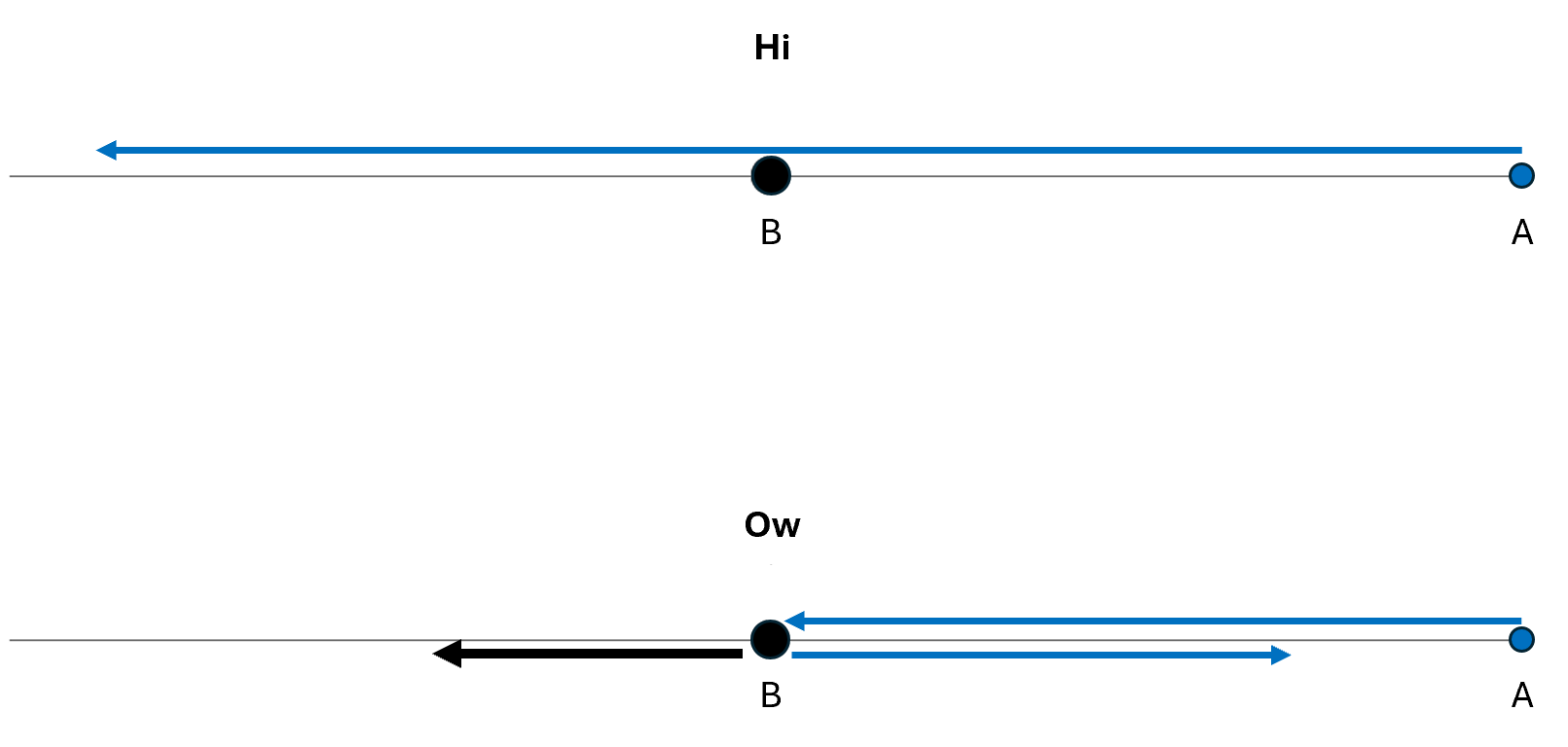
Or, using an animation, we can show the time-dependence more explicitly and more clearly. In the second case, I’ve assumed that B has more mass than A, so it recoils more slowly from the blow than does A.


Motion in the Two-Dimensional Space of Possibilities
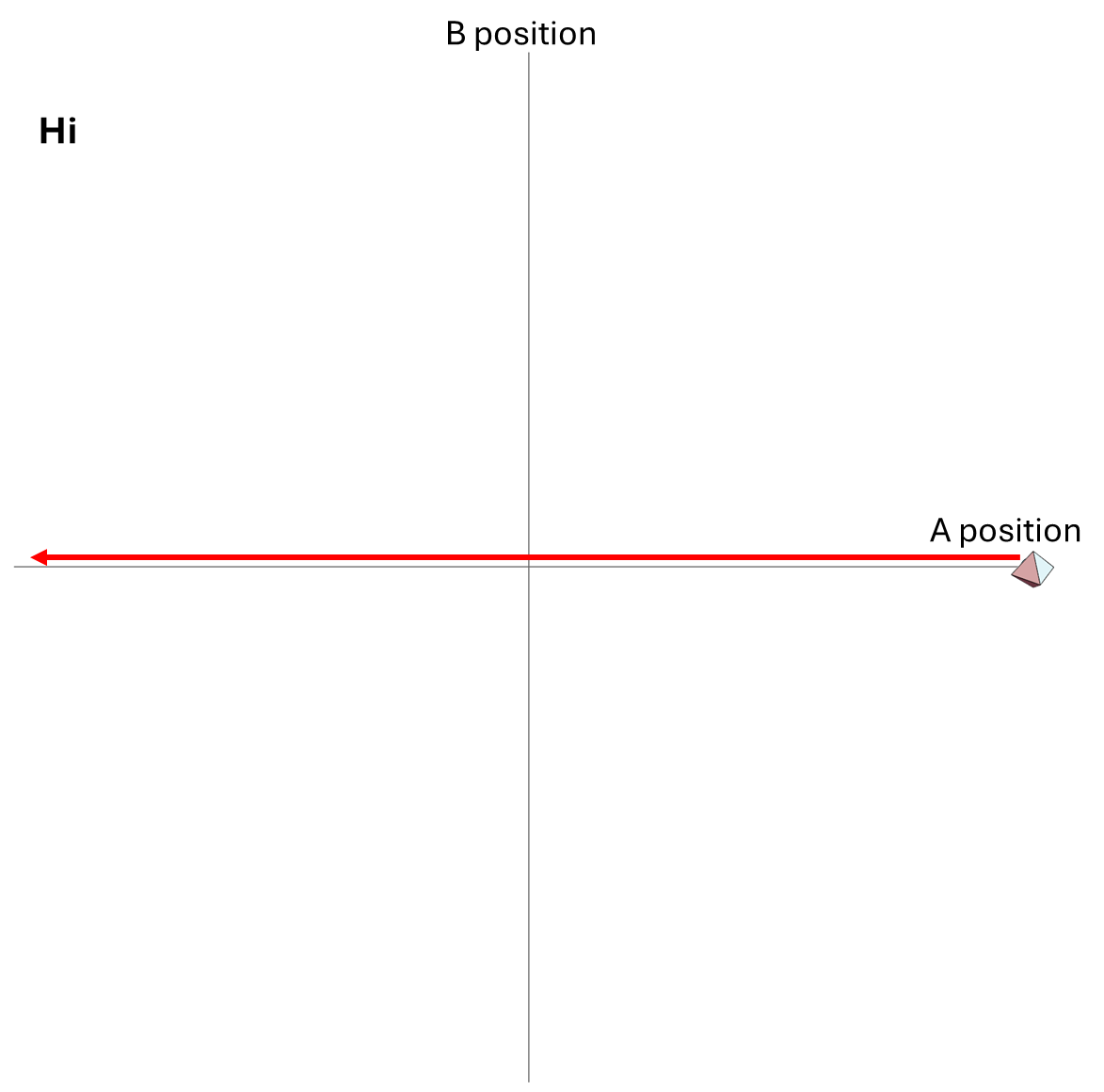
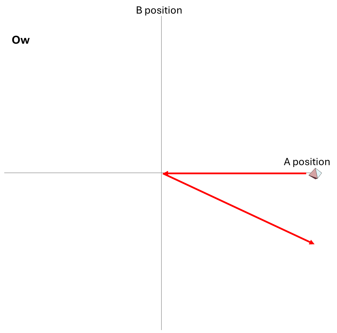
But we could also describe how the particles move as a system in their two-dimensional space of possibilities. Each point in that space tells us both where A is and where B is; the point’s location along the horizontal axis gives A’s position, and its location along the vertical axis gives B’s position. At each moment, the system is at one point in that space; over time, as A and B change their positions, the location of the system in that two-dimensional space also changes.
The motion of the system for the Hi and Ow cases is shown in Fig. 3. It has exactly the same information as Fig. 1, though depicted differently and somewhat more precisely. Instead of following the two dots that correspond to the two particles as they move in one dimension, we now depict the whole system as a single diamond that tells us where both particles are located.
In the first part of Fig. 3, we see that B’s position is at the center of the space, and remains there, while A’s position goes from the far right to the far left; compare to Fig. 1. In the second part of Fig. 3, A and B collide at the center, following which A moves to positive position, B moves to negative position, and correspondingly, within its space of possibilities, the system as a whole moves down and to the right.
And finally, let’s look at an animation in the two-dimensional space of possibilities. Compare this to Fig. 3, and then to Fig. 2, noting that it has the same information.

In Fig. 4, we see that
- the system as a whole is represented as a single moving point in the space of possibilities
- each of the two futures for the system are represented as separate time-dependent paths across the space of possibilities
The Quantum System
Now, what if the system is described using quantum physics? What’s up with the system’s wave function?
As noted, we do not have a wave function for particle A and a separate wave function for particle B, and so we do not have a collision of two wave functions. Instead, we have a single wave function for the A/B system, one which describes the collision of the two particles and the aftermath thereof.
It is impossible to depict the wave function using the one-dimensional universe that the particles live in. The wave function itself only exists in the space of possibilities. So in quantum physics, there are no analogues to Figs. 1 and 2.
Meanwhile, although we can depict the wave function at any one moment in the two dimensional space, we cannot simply use arrows to depict how it changes over time. This is because we cannot view the “Hi” and “Ow” cases as distinct, and as something we can draw in two separate figures, as we did in Figs. 3 and 4. In quantum physics, we have to view both possibilities as described by the same wave function; they are not distinct outcomes.
The only option we have is to do an animation in the two-dimensional space of possibilities, somewhat similar to Fig. 4, but without separating the Hi and Ow outcomes. There’s just one wave function that shows both the “Hi” and “Ow” cases together. The square of this wave function, which gives the probabilities for the system’s possible futures, is sketched in Fig. 5.
[Note that what is shown is merely a sketch! It is not the true wave function, which requires a complete solution of Schrödinger’s wave equation. While the solution is well known, it is tricky to get all the details of the math exactly right, and I haven’t had the time. I’ll try to add the complete and correct solution at a later date.]
Compare Fig. 5 with Fig. 4, recalling that the probability of the Hi case is 30% and the probability of the Ow case is 70%. Both possibilities appear in the wave function, with the branch corresponding to the Ow case carrying larger weight than the branch corresponding to the Hi case.
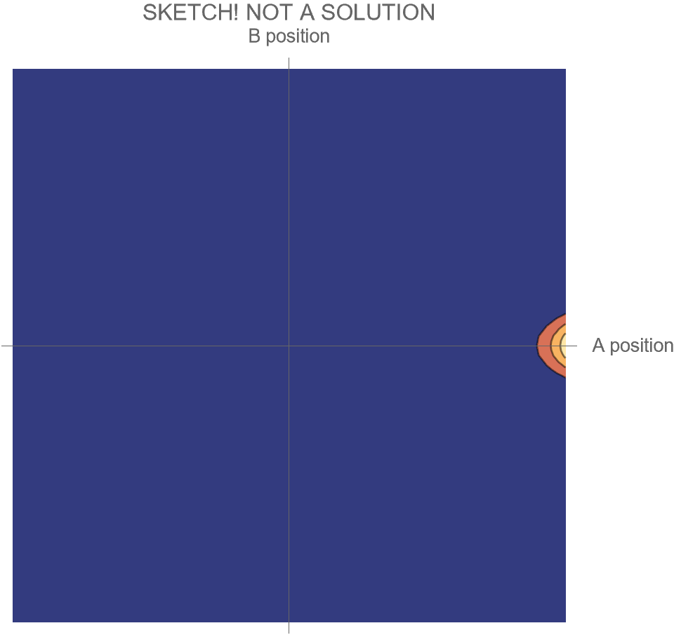
In contrast to Fig. 4, the key differences are that
- the system is no longer represented as a point in the space of possibilities, but instead as a (broadened) set of possibilities
- the wave function is complicated during the collision, and develops two distinct branches only after the collision
- all possible futures for the system exist within the same wave function
- this has the consequence that distinct future possibilities of the system could potentially affect each other at a later time — a concept which makes no sense in non-quantum physics
- the probabilities of those distinct futures are given by the relative sizes of the wave function within the two branches.
Notice that even though particle A has a 70% probability of “hurting” B, the wave function itself does not, and cannot, “hurt” B. It just describes what may happen; it contains both A and B, and describes both the possibility of Hi and Ow. The wave function isn’t a part of the A/B system, and doesn’t participate in its activities. Instead, it exists outside the system, as a means for understanding that system’s behavior.
Summing Up
A system has a wave function, but individual objects in the system do not have wave functions. That’s the key point.
To be fair, it is true that when objects or groups of objects in a system interact weakly enough, we may imagine the system’s full wave function as though it were a simple combination of wave functions for each object or group of objects. That is true of the initial Schrödinger cat wave function, which is a product of separate factors for the atom, device and cat, and is also true of the wave function in Fig. 5 before the collision of A and B. But once significant interactions occur, this is no longer the case, as we see in the later-stage Schrödinger cat wave function and in Fig. 5 after the collision.
A wave function expresses how the overall system moves through the full space of its possibilities, and grows ever more complex when there are many possible paths for a system to take. This is completely unrelated to wavicles, which are objects that move through physical space and create physical phenomena, forming parts of a system that itself is described by a wave function.
A Final Note on Wave Functions
As a final comment: I’ve given this simple example because it’s one of the very few that one can draw start to finish.
Wave functions of systems with just one particle are misleading, because they make it easy to imagine that there is one wave function per particle. But with more than one particle, the only wave functions that can easily be depicted are those of two particles moving in one dimension, such as the one I have given you. Such examples offer a unique opportunity to clarify what a wave function is and isn’t, and it’s therefore crucial to appreciate them.
Any wave function more complicated than this becomes impossible to draw. Here are some things to consider.
- I have only drawn the square of the wave function in Fig. 5. The full wave function is a complex function (i.e. a complex number at each point in the space of possibilities), and the contour plot I have used in Fig. 5 could only be used to draw its real part, its imaginary part, or its square. Thus even in this simple situation with a two-dimensional space of possibilities, the full wave function cannot easily be represented.
- If we had four particles moving in one dimension instead of two, with positions x1, x2, x3 and x4 respectively, then the wave function would be a function of the four-dimensional space of possibilities, with coordinates x1, x2, x3, x4 . [The square of the wave function at each point in that space tells us the probability that particle 1 is at position x1, particle 2 is at position x2, and similarly for 3 and 4.] A function in four dimensions can be handled using math, but is impossible to draw.
- If we had two particles moving in three dimensions, the first with position x1, y1, z1, and the second with position x2, y2, z2, the space of possibilities would be six-dimensional — x1, y1, z1, x2, y2, z2 . Again, this cannot be drawn.
These difficulties explain why one almost never sees a proper discussion of wave functions of complicated systems, and why wave functions of fields are almost never described and are never depicted.